© 2008--2013 Krishna Myneni

R is a free and powerful computing environment, designed for numerical computations and visualizing data. It is available for a wide variety of systems, and may be obtained from http://www.r-project.org. R is also a language for expressing, and programming numerical calculations. The language of R is object-oriented and elegant, with a simple and intuitive syntax. While many of the built-in functions of R are useful for performing calculations in statistics, the large variety of functions, as well as package extensions, allow R to be applied to a wide range of problems in the physical sciences and applied mathematics. These notes illustrate some common computational tasks encountered by students, teachers, and researchers in the physical sciences.
	R version 2.6.2 (2008-02-08)
	Copyright (C) 2008 The R Foundation for Statistical Computing
	ISBN 3-900051-07-0

	R is free software and comes with ABSOLUTELY NO WARRANTY.
	You are welcome to redistribute it under certain conditions.
	Type 'license()' or 'licence()' for distribution details.

	  Natural language support but running in an English locale

	R is a collaborative project with many contributors.
	Type 'contributors()' for more information and
	'citation()' on how to cite R or R packages in publications.

	Type 'demo()' for some demos, 'help()' for on-line help, or
	'help.start()' for an HTML browser interface to help.
	Type 'q()' to quit R.

	>
> source("filename")
where filename is the name of a file, typically with extension .R, containing the R commands to be executed.
> help("seq")
If you are unsure of the exact function name, you may also search the documentation
for a particular topic, using help.search. For example,
> help.search("sequence")
will show relevant functions for sequence generation.
	> myfunc <- function(x) {
      		y <- cos(x) + sin(x)
      		return (y)
  	}
	>
	> myfunc(0.5)
	[1] 1.357008
	>
	> myfunc(0.5*1i)
	[1] 1.127626+0.521095i
	>
	> myfunc(-2 + 5*1i)
	[1] -98.36115+36.59336i
	>
	> x <- seq(-4, 4, by=0.01)
	> y <- myfunc(x)
x is a vector, generated by the seq function. It may be passed as an argument to the function, and a vector, y, is returned. Assignment of the variables x and y may also be done with the more conventional notation,
	> x = seq(-4, 4, by=0.01)
	> y = myfunc(x)
> plot(myfunc, 0, 2*pi)
> plot(myfunc2, 0, 2*pi, add=TRUE)
> plot(myfunc2, 0, 2*pi, add=TRUE, col="red")
We will take as an example, the problem of finding the roots
of the function,
          f(x) = f_g(x) - f_l(x)


where

          f_g(x) = exp(-a*x^2)

and

          f_l(x) = b/(x^2 + b)
For the example, we will take a=1, b=0.5.The problem of finding the roots of f(x) is the same as the problem of finding the values of x at which the two functions, f_g(x) and f_l(x), intersect. The problem can be solved approximately by plotting the two functions, and visually determining the values of x at which they intersect --- the graphical method. A more precise method is to use an iterative search of $x$, to find the values at which f(x) = 0. R provides such a search method with the function uniroot. However, we must first obtain the approximate roots with the graphical method, so that the search interval can be bounded for uniroot.
      > a = 1
      > b = 0.5
Define the functions, f_g(x), and f_l(x), and plot them
together on a graph:
      > fg <- function(x) { return( exp(-a*x^2) ) }
      > fl <- function(x) { return( b/(x^2 + b) ) }
      > plot(fg, -5, 5, col='blue')
      > plot(fl, -5, 5, col='red', add=TRUE)
The following graph will appear.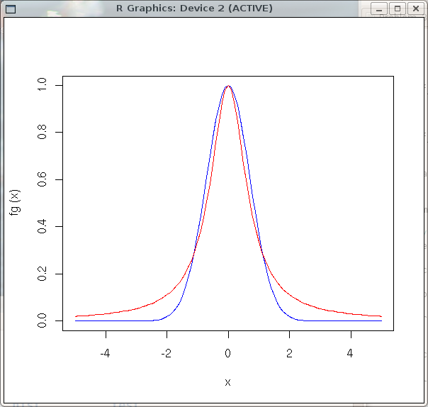
> f <- function(x) { return( fg(x) - fl(x) ) }
Now, find the precise value of a given root (value of x at which
fg(x) and fl(x) intersect), using its approximate vicinity. From
the graphical method, we know there is a root near x = -1. Using uniroot,
a precise value may be found by specifying the interval in x over which
to search for the root,> uniroot(f, c(-1.2, -0.8)) $root [1] -1.120907 $f.root [1] -4.398283e-08 $iter [1] 3 $estim.prec [1] 0.0001094043uniroot searches for the root in the interval, x = (-1.2, -0.8), and outputs several values: the root itself, the value of the function f at the root position, the number of iterations required to find the root, and the estimated precision of the root. From the output above, we see that this root occurs at
	> root1 = uniroot(f, c(-1.2, -0.8))$root
	> root1
	[1] -1.120907
> z <- 3.2+4*1ior
> z = 3.2+4*1i
	> Re(z)
	[1] 3.2
	> Im(z)
	[1] 4
	> Mod(z)
	[1] 5.122499
	> abs(z)
	[1] 5.122499
	> Arg(z)
	[1] 0.8960554
The Mod and abs functions both return the length (modulus) of the number, and Arg returns the argument (phase).
	> x = 3 + 1i*2
	> Conj(x)
	[1] 3-2i
	>
	> x <- c(1, 2, 3, 11, 12, 13)
	> x
	[1]  1  2  3 11 12 13
	>
	> mat1 <- matrix(c(1,2,3,11,12,13), nrow=2, byrow=TRUE)
	> mat1
	     [,1] [,2] [,3]
	[1,]    1    2    3
	[2,]   11   12   13
	>
	> mat2 <- matrix(c(1+1i, 0, 0, 1-1i), nrow=2, byrow=TRUE)
	> mat2
	     [,1] [,2]
	[1,] 1+1i 0+0i
	[2,] 0+0i 1-1i
	>
       > x <- seq(-4, 4, by=0.01)
       > length(x)
       [1] 801
shows that we have created an 801 element vector using the seq function.
       > mat1 <- matrix(c(1,2,3,11,12,13), nrow=2, byrow=TRUE)
       > dim(mat1)
       [1] 2 3
dim returns a vector containing the dimensions of the matrix.
       > x <- 1:10
       > x
       [1]  1  2  3  4  5  6  7  8  9 10
       > y <- 11:20
       > y
       [1] 11 12 13 14 15 16 17 18 19 20
       > z <- c(x, y)
       > z
       [1]  1  2  3  4  5  6  7  8  9 10 11 12 13 14 15 16 17 18 19 20
In the above example, the vectors x and y are 10 element
vectors. The combine function, c(), is used to combine (concatenate) the
elements together to form the vector, z.
       > x <- seq(-2, 2, by=0.1)
       > length(x)
       [1] 41
       > y <- x[18:24]
       > y
       [1] -0.3 -0.2 -0.1  0.0  0.1  0.2  0.3
In this example, we create a 41 element vector, x, and use the range
18:24, to specify the index range for elements in x, which
are returned to form the new vector y.
	> x <- seq(-4, 4, by=0.01)
	> y <- myfunc(x)
	> d <- array(c(x,y), c(length(x), 2))
x and y are vectors (1-d arrays), generated from a sequence, and a function, respectively.
d is a 2-column matrix, with column 1 containing x, and column 2 containing y.
	> x <- d[,1]
	> y <- d[,2]
The first column of matrix d is placed in vector x, and the second column of d is placed in vector y.
> d <- scan("filename")
> d <- matrix(scan("filename"), ncol=2, byrow=TRUE)
> write(x, ncolumns=1, file="array.dat")
> write(t(mat1), ncolumns=3, file="matrix.dat")Notice the use of the transpose function, t(). The matrix must be transposed, using t(), to make the columns in the file correspond to the columns of the matrix.
	> x <- seq(-4, 4, by=0.01)
	> y <- myfunc(x)
	> plot(x,y)
x and y are vectors of the same length.
	> d <- array(c(x,y), c(length(x), 2))
 	> plot(d)
> plot(d, type="l", col="red", xlab="Time (s)", ylab="Vout (V)")
Other plot attributes such as title, xlim, and ylim may also be specified.
	> plot(d, xlim=c(-4, 4), ylim=c(-1,1))
	> lines(x, y, col="blue")
	> lines(d2, col="green")
The first plot command sets up the graph and plots the matrix d. Subsequent lines commands overlays plots of the respective data onto the graph.
	> a <- matrix(c(1, 0, -2, 0, 3, -1), nrow=2, byrow=TRUE)
	> b <- matrix(c(0, 3, -2, -1, 0, 4), nrow=3, byrow=TRUE)
	> c <- a%*%b
	> c
     		[,1] [,2]
	[1,]    0   -5
	[2,]   -6   -7
	> d <- b%*%a
	> d
     		[,1] [,2] [,3]
	[1,]    0    9   -3
	[2,]   -2   -3    5
	[3,]    0   12   -4
	>
	> a <- matrix(c(1, 0, -2, 4, 1, 0, 1, 1, 7), nrow=3, byrow=TRUE)
	> a
     		[,1] [,2] [,3]
	[1,]    1    0   -2
	[2,]    4    1    0
	[3,]    1    1    7
	> b <- solve(a)
	> b
     		[,1] [,2] [,3]
	[1,]    7   -2    2
	[2,]  -28    9   -8
	[3,]    3   -1    1
	>
	> a <- matrix(c(1, 0, -2, 4, 1, 0, 1, 1, 7), nrow=3, byrow=TRUE)
	> sum(diag(a))
        [1] 9
The diag function retrieves the diagonal elements of the matrix.
	> sigma_x <- matrix(c(0,1,1,0), nrow=2, byrow=TRUE)
	> sigma_x
	     [,1] [,2]
	[1,]    0    1
	[2,]    1    0
	> eigen(sigma_x)
	$values
	[1]  1 -1

	$vectors
	          [,1]       [,2]
	[1,] 0.7071068 -0.7071068
	[2,] 0.7071068  0.7071068

	>
	> Jy <- matrix(c(0,1,0,-1,0,1,0,-1,0), nr=3, byrow=TRUE)
	> Jy
	     [,1] [,2] [,3]
	[1,]    0    1    0
	[2,]   -1    0    1
	[3,]    0   -1    0
	> Jy <- Jy*(0+1i)/sqrt(2)
	> Jy
	             [,1]         [,2]         [,3]
	[1,] 0+0.0000000i 0+0.7071068i 0+0.0000000i
	[2,] 0-0.7071068i 0+0.0000000i 0+0.7071068i
	[3,] 0+0.0000000i 0-0.7071068i 0+0.0000000i
	> eigen(Jy)
	$values
	[1]  1.000000e+00 -2.376571e-16 -1.000000e+00

	$vectors
	                [,1]                       [,2]            [,3]
	[1,] -0.5+0.0000000i 7.071068e-01+0.000000e+00i -0.5+0.0000000i
	[2,]  0.0+0.7071068i 0.000000e+00+2.498002e-16i  0.0-0.7071068i
	[3,]  0.5+0.0000000i 7.071068e-01+0.000000e+00i  0.5+0.0000000i

	>
Visit http://cran.r-project.org and click on Packages. An alphabetical list of available packages for R will be displayed. Click on a particular package name to obtain additional information about the package, including a pdf document which describes its use.
It is not necessary to download the package source for installation if the machine on which you installed R has internet access.
> install.packages()A list of mirror sites for R packages will appear. Select an appropriate mirror site. Then a list of available packages will appear. Select the desired package. The package will be downloaded, built, and installed.
From within the R environment, or within an R script, you may load a package using,
> require("packagename")
We will use the extra R package deSolve to illustrate how to solve a system of ordinary
differential equations. This package provides the robust ODE solver named lsoda taken from
the well-known collection of solvers, ODEPACK, written by Alan Hindmarsh and others. Assuming that
you have installed the deSolve package using the procedure given above, you may use it
to find a solution to the following system of first order differential equations:
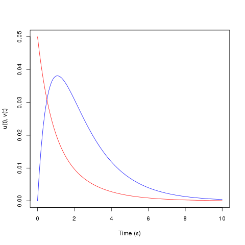
	du/dt = -u + alpha*v

	dv/dt = beta*u - v
where alpha and beta are two specified parameters. Although the above set of coupled, linear, first-order differential equations may be solved easily by linear methods, they are used to illustrate the general numerical procedure, which may be applied to a more complex system of linear or nonlinear differential equations.
First, define a function which computes the derivatives, given the current values of the variables,
the independent variable (time, for example), and the values of the parameters:
# Function to evaluate the ODEs

derivs <- function(t, x, p) {
	udot = -x[1] + p[1]*x[2]
	vdot = p[2]*x[1] - x[2]
	return (list(c(udot, vdot)))
}
The function named derivs takes three arguments: the value of the independent variable (time),
a vector x containing the state of the system at the current time, and a vector containing the
parameter values. Thus, at the current value of t,u = x[1] v = x[2] alpha = p[1] beta = p[2]and derivs returns a list of the values of the derivatives. In order to compute a numerical solution of the equations using lsoda, we must supply it with a vector of time values for which we want the solution, and the initial conditions, i.e. the values of the variables at the starting time. The vector of parameter values must also be specified. Thus, we must do the following:
params <- c( 2, 0.1 )              # alpha = 2, beta = 0.1
x0 <- c(0, 0.05)                   # initial conditions
times <- c(0, 0.1*(1:100))         # time steps at which to compute the solution

require("deSolve")

# Solve the differential equations for this example
out <- lsoda( x0, times, derivs, params)
The solutions, u(t) and v(t), are stored in the array out. They
may be plotted using the following commands.> plot(out[,1], out[,2], type='l', col="blue", xlab="Time (s)", ylab="u(t), v(t)", ylim=c(0, .05)) > lines(out[,1], out[,3], col="red")The following graph will be shown.